社会主義は帰ってくるのか
21世紀によみがえる「大きな政府」
2019.2.22（金） 池田 信夫
バーニー・サンダース氏、20年米大統領選出馬に「脈あり」
米首都ワシントンで講演するバーニー・サンダース上院議員（2017年6月22日撮影、資料写真）。(c)Mandel Ngan / AFP〔AFPBB News〕

　2020年に行われるアメリカの大統領選挙に、バーニー・サンダース上院議員が出馬を表明した。彼は2016年の大統領選挙で、ヒラリー・クリントン上院議員と最後まで民主党の候補を争ったことで知られる。彼の掲げる政策は、国民皆保険、全米最低賃金15ドル、公立学校の無償化など、巨額の財源を必要とする「大きな政府」である。

　サンダースはみずから「民主社会主義者」と名乗り、民主党左派に大きな支持を集めている。社会主義は20世紀に崩壊し、過去のものになったと思われているが、サンダースを支持するのは、冷戦の終了後に生まれた若者だ。時代は一めぐりして、社会主義の時代がやってくるのだろうか。

財源の不明な「グリーン・ニューディール」
　サンダースの選挙運動の中心になっているのが、アレクサンドリア・オカシオ＝コルテス下院議員である。昨年（2018年）初当選したばかりでまだ29歳だが、彼女も民主社会主義者を名乗っている。

　彼女は「グリーン・ニューディール」（GND）という大胆なエネルギー政策を提案して注目を集めた。これは「今後10年以内に全米のエネルギーを100％再生可能エネルギーに変える」という決議案で、ベーシック・インカム（すべての人に定額の所得を保障する）や国民皆保険などの「格差是正計画」も入っている。

　この決議案には法的拘束力はないが、大統領候補に名乗りを上げた政治家のうち6人がこの決議案に署名した。こういう突飛な案が議会で議論される背景には、アメリカの格差が拡大している状況がある。アメリカでは所得の20％が人口の1％の富裕層に集中し、最貧層との格差が大きな社会問題になっている。

　10年で全米の火力発電所や原子力発電所をすべて廃止して再エネに変えるには、年間3兆ドル（330兆円）以上のコストがかかるといわれる。ベーシック・インカムにも同じぐらいの財源が必要で、GNDのコストは連邦政府の予算をはるかに上回る。

　その財源はどうするのだろうか。サンダースは金持ちの資産に「富裕税」をかけると主張し、オカシオ＝コルテスは所得税の最高税率を70％に引き上げるというが、そんな大増税が簡単にできるとは思えない。そのとき財源はどうするのか。

政府の借金は紙幣を印刷してまかなう
　紙幣を印刷すればいい、というのがオカシオ＝コルテスの答である。これはMMT（modern monetary theory）というあやしげな経済理論で、「国債はお札を印刷してファイナンスできるので、財政は破綻しない」という。これが本当なら、増税しないで政府支出をいくらでも増やせる「フリーランチ」があることになる。

　政府債務が増えると金利が上がり、それによって（元利合計した）政府債務が増え、それによって国債のリスクが高まり、それによって金利が上がる・・・という悪循環に入り、「財政インフレ」で政府債務が無限大に発散するというのが経済学の常識だ。

　しかし今のような超低金利が今後もずっと続くとすれば、財政が破綻する心配はない。日本でも国債が増発され、日銀がそれを400兆円以上買っても金利は下がる一方で、最近は長期金利もほぼゼロという世界史に前例のない低水準である。

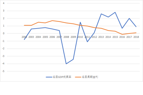
　単純化していうと、名目金利が名目成長率を下回る限り、政府債務は発散しない。これは成長率が高いと税収の伸びが金利負担の伸びを上回るからだ。下の図のように2013年以降は金利が成長率より低いので、この状況が今後もずっと続くなら、フリーランチはありうる。

http://jbpress.ismedia.jp/mwimgs/6/f/500/img_6f8b492feed47a189cb61e3c1d8b42b013123.png
名目成長率と名目金利（％、内閣府調べ）

ゼロ金利はいつまで続くのか

　財政が破綻しないとしても、今の世代が借金して将来世代がそれを返すのは、負担を子孫に先送りすることになるのではないか。これはもっともな疑問だが、国債のほとんどは日本国民が買うので、国民の資産でもある。国債がすべて相続されると将来世代の資産が増えるので、国民全体としては同じだ（所得分配は無視する）。

　これは名目ベースの話で、実質的な負担は金利と成長率の関係によって違う。たとえば金利が1％だとすると、借金は20年後には元利合計で約1.2倍になるが、成長率が2％だとGDPは20年後には約1.5倍になる。つまり金利が成長率より低いと、将来世代の借金返済の負担（GDP比）は軽くなるので、いま借金して将来返したほうが国民全体として有利になるのだ。

　逆に金利が成長率より高いと、将来世代の負担は重くなる。彼らの損失は、政府の借金が民間投資を押しのけることによって生じる資本蓄積の減少だから、金利（資本収益率）が成長率より低いときは、民間に代わって政府が投資することが効率的だ。直感的にいうと、ゼロ金利が今後もずっと続くなら貯金しても資産は増えないので、いま政府が使ったほうがいいのだ（＊）。

　これはアメリカでは重要な問題で、社会保障のインフラを政府が整備すべきかどうかについて長い論争がある。その財源を増税でまかなうことには共和党が反対しているので政治的に不可能だが、国債の増発は政治的には容易である。

　ヨーロッパでも2010年代にEU（ヨーロッパ連合）が南欧諸国の財政危機を支援する条件として緊縮財政を強要したことに反発して「反緊縮」の運動が強まった。

　日本では一足先に、安倍政権が「大きな政府」に舵を切った。日本の政府債務はGDP比で世界最悪だが、安倍首相は2度も増税を延期し、日銀が財政ファイナンスで国債を買い支えている。多くの経済学者は「国債が暴落する」と警告してきたが、実質金利はほぼゼロになった。何かが変わったのではないか、と主流の経済学者も考え始めた。

　しかし何が変わったのか、原因は分からない。日本が2000年代にゼロ金利になったとき、世界の経済学者が日銀の金融政策を嘲笑したが、今は世界にゼロ金利が広がっている。これが今後も続くかどうかも分からないので、財政赤字を膨張させることは危険だが、「大きな政府か小さな政府か」についての論争には、まだ答が出ていないのである。

（＊）この話はいろいろな条件を単純化しているので、厳密な議論は今年1月のアメリカ経済学会長講演を読んでいただきたい。
http://jbpress.ismedia.jp/articles/-/55571

　
https://www.aeaweb.org/aea/2019conference/program/pdf/14020_paper_etZgfbDr.pdf
Public Debt and Low Interest Rates
By Olivier Blanchard ∗
The lecture focuses on the costs of public debt when safe interest
rates are low. I develop four main arguments.
First, I show that the current U.S. situation in which safe interest
rates are expected to remain below growth rates for a long time,
is more the historical norm than the exception. If the future is
like the past, this implies that debt rollovers, that is the issuance
of debt without a later increase in taxes may well be feasible. Put
bluntly, public debt may have no fiscal cost.
Second, even in the absence of fiscal costs, public debt reduces capital accumulation, and may therefore have welfare costs. I show
that welfare costs may be smaller than typically assumed. The
reason is that the safe rate is the risk-adjusted rate of return on
capital. If it is lower than the growth rate, it indicates that the
risk-adjusted rate of return to capital is in fact low. The average
risky rate however also plays a role. I show how both the average
risky rate and the average safe rate determine welfare outcomes.
Third, I look at the evidence on the average risky rate, i.e. the
average marginal product of capital. While the measured rate of
earnings has been and is still quite high, the evidence from asset
markets suggests that the marginal product of capital may be lower,
with the difference reflecting either mismeasurement of capital or
rents. This matters for debt: The lower the marginal product, the
lower the welfare cost of debt.
Fourth, I discuss a number of arguments against high public debt,
and in particular the existence of multiple equilibria where investors believe debt to be risky and, by requiring a risk premium,
increase the fiscal burden and make debt effectively more risky.
This is a very relevant argument, but it does not have straightforward implications for the appropriate level of debt.
My purpose in the lecture is not to argue for more public debt,
especially in the current political environment. It is to have a
richer discussion of the costs of debt and of fiscal policy than is
currently the case.
∗ Peterson Institute for International Economics and MIT (oblanchard@piie.com) AEA Presidential Lecture, to be given in January 2019. Special thanks to Larry Summers for many discussions and
many insights. Thanks for comments, suggestions, and data to Laurence Ball, Simcha Barkai, Charles
Bean, Philipp Barrett, Ricardo Caballero, John Campbell, John Cochrane, Carlo Cottarelli, Peter Diamond, Stanley Fischer, Francesco Giavazzi, Robert Hall, Patrick Honohan, Anton Korinek, Larry Kotlikoff, Lorenz Kueng, Neil Mehrotra, Jonathan Parker, Thomas Philippon, Jim Poterba, Ricardo Reis,
Dmitriy Sergeyev, Jay Shambaugh, Robert Solow, Jaume Ventura, Philippe Weil, Ivan Werning, Jeromin
Zettelmeyer, and many of my PIIE colleagues. Thanks for outstanding research assistance to Thomas
1
2 THE AMERICAN ECONOMIC REVIEW MONTH YEAR
I. Introduction
Since 1980, interest rates on U.S. government bonds have steadily decreased.
They are now lower than the nominal growth rate, and according to current
forecasts, this is expected to remain the case for the foreseeable future. 10-year
U.S. nominal rates hover around 3%, while forecasts of nominal growth are around
4% (2% real growth, 2% inflation). The inequality holds even more strongly in
the other major advanced economies: The 10-year UK nominal rate is 1.3%,
compared to forecasts of 10-year nominal growth around 3.6% (1.6% real, 2%
inflation). The 10-year Euro nominal rate is 1.2%, compared to forecasts of
10-year nominal growth around 3.2% (1.5% real, 2% inflation).1 The 10-year
Japanese nominal rate is 0.1%, compared to forecasts of 10-year nominal growth
around 1.4% (1.0% real, 0.4% inflation).
The question this paper asks is what the implications of such low rates should
be for government debt policy. It is an important question for at least two reasons.
From a policy viewpoint, whether or not countries should reduce their debt, and
by how much, is a central policy issue. From a theory viewpoint, one of pillars
of macroeconomics is the assumption that people, firms, and governments are
subject to intertemporal budget constraints. If the interest rate paid by the
government is less the growth rate, then the intertemporal budget constraint
facing the government no longer binds. What the government can and should do
in this case is definitely worth exploring.
The paper reaches strong, and, I expect, surprising, conclusions. Put (too)
simply, the signal sent by low rates is that not only debt may not have a substantial
fiscal cost, but also that it may have limited welfare costs.
Given that these conclusions are at odds with the widespread notion that government debt levels are much too high and must urgently be decreased, the paper
considers several counterarguments, ranging from distortions, to the possibility
that the future may be very different from the recent past, to multiple equilibria.
All these arguments have merit, but they imply a different discussion from that
dominating current discussions of fiscal policy.
The lecture is organized as follows.
Section 1 looks at the past behavior of U.S. interest rates and growth rates. It
concludes that the current situation is actually not unusual. While interest rates
on public debt vary a lot, they have on average, and in most decades, been lower
than growth rates. If the future is like the past, the probability that the U.S.
government can do a debt rollover, that is issue debt and achieve a decreasing
debt to GDP ratio without ever having to raise taxes later is high.
That debt rollovers may be feasible does not imply however that they are desirable. Even if higher debt does not give rise later to a higher tax burden, it
Pellet, Colombe Ladreit, and Gonzalo Huertas. Appendices and data sources: https://bit.ly/2xSSw9O
1Different Euro countries have different government bond rates. The 10-year Euro nominal rate
is a composite rate (with changing composition) constructed by the ECB.http://sdw.ecb.europa.eu/
quickview.do?SERIES_KEY=143.FM.M.U2.EUR.4F.BB.U2_10Y.YLD
VOL. VOLUME NO. ISSUE DEBT AND RATES 3
still has effects on capital accumulation, and thus on welfare. Whether and when
higher debt increases or decreases welfare is taken up in Sections 2 and 3.
Section 2 looks at the effects of an intergenerational transfer (a conceptually
simpler policy than a debt rollover, but a policy that shows most clearly the relevant effects at work) in an overlapping generation model with uncertainty. In
the certainty context analyzed by Diamond (1965), whether such an intergenerational transfer from young to old is welfare improving depends on “the” interest
rate, which in that model is simply the net marginal product of capital. If the
interest rate is less than the growth rate, then the transfer is welfare improving.
Put simply, in that case, a larger intergenerational transfer, or equivalently an
increase in public debt, and thus less capital, is good.
When uncertainty is introduced however, the question becomes what interest
rate we should look at to assess welfare effects of such a transfer. Should it be
the average safe rate, i.e. the rate on sovereign bonds (assuming no default risk),
or should it be the average marginal product of capital? The answer turns out to
be: Both.
As in the Diamond model, a transfer has two effects on welfare, an effect through
reduced capital accumulation, and an indirect effect, through the induced change
in the returns to labor and capital.
The welfare effect through lower capital accumulation depends on the safe rate.
It is positive if, on average, the safe rate is less than the growth rate. The intuitive
reason is that, in effect, the safe rate is the relevant risk-adjusted rate of return
on capital, thus it is the rate that must be compared to the growth rate.
The welfare effect through the induced change in returns to labor and capital
depends instead on the (risky) marginal product of capital. It is negative if, on
average, the marginal product of capital exceeds the growth rate.
Thus, in the current situation where it indeed appears that the safe rate is less
than the growth rate, but the average marginal product of capital exceeds the
growth rate, the two effects have opposite signs, and the effect of the transfer on
welfare is ambiguous. The section ends with an approximation which shows most
clearly the relative role of the two rates. The net effect may be positive, if the
safe rate is sufficiently low, and the average marginal product is not too high.
With these results in mind, Section 3 turns to numerical simulations. People
live for two periods, working in the first, and retiring in the second. They have
separate preferences vis-a-vis intertemporal substitution and risk. This allows to
look at different combinations of risky and safe rates, depending on the degree
of uncertainty and the degree of risk aversion. Production is CES in labor and
capital, and subject to technological shocks: Being able to vary the elasticity of
substitution between capital and labor turns out to be important as this elasticity
determines the strength of the second effect on welfare. There is no technological
progress, nor population growth, so the average growth rate is equal to zero.
I show how the welfare effects of a transfer can be positive or negative, and
how they depend in particular on the elasticity of substitution between capital
4 THE AMERICAN ECONOMIC REVIEW MONTH YEAR
and labor. In the case of a linear technology (equivalently, an infinite elasticity
of substitution between labor and capital), the rates of return, while random, are
independent of capital accumulation, so that only the first effect is at work, and
the safe rate is the only relevant rate in determining the effect of the transfer
on welfare. I then show how a lower elasticity of substitution implies a negative
second effect, leading to an ambiguous welfare outcome.
I then turn to debt and show that a debt rollover differs in two ways from
a transfer scheme. First, with respect to feasibility. So long as the safe rate
remains less than the growth rate, the ratio of debt to GDP decreases over time;
a sequence of adverse shocks may however increase the safe rate sufficiently so
as to lead to explosive dynamics, with higher debt increasing the safe rate, and
the higher safe rate in turn increasing debt over time. Second, with respect to
desirability: A successful debt rollover can yield positive welfare effects, but less
so than the transfer scheme. The reason is that a debt rollover pays people a
lower rate of return than the implicit rate in the transfer scheme.
The conclusions, and the welfare effects of debt in Section 3 depend not only
how on low the average safe rate is, but also how high the average marginal
product is. With this in mind, Section 4 returns to the empirical evidence on the
marginal product of capital. It focuses on two facts. The first fact is that the
ratio of the earnings rate of U.S. corporations to their capital at replacement cost
has remained high and relatively stable over time. This suggests a high marginal
product, and thus, other things equal, a higher welfare cost of higher debt. The
second fact, however, is that the ratio of the earnings of U.S. corporations to their
market value has substantially decreased since the early 1980s. Put another way,
Tobin‘s q, which is the ratio of the market value of capital to the value of capital
at replacement cost, has substantially increased. Two potential interpretations
are that capital at replacement cost is poorly measured and does not fully capture
intangible capital. The other is that an increasing proportion of earnings comes
from rents. Both explanations (which are the subject of much current research)
imply a lower marginal product for a given measured earnings rate, and thus a
smaller welfare cost of debt.
Section 5 goes beyond the formal model and places the results in a broader but
informal discussion of the costs and benefits of public debt.
On one side, the model above has looked at debt issuance used to finance
transfers in a full employment economy; this does not do justice to current policy
discussions, which have focused on the role of debt finance to increase demand
and output if the economy is in recession, and on the use of debt to finance public
investment. This research has concluded that, if the neutral rate of interest is low
and the effective lower bound on interest rates is binding, then there is a strong
argument for using fiscal policy to sustain demand. The analysis above suggests
that, in that very situation, the fiscal and welfare costs of higher debt may be
lower than has been assumed, reinforcing the case for a fiscal expansion.
On the other side, (at least) three arguments can be raised against the model
VOL. VOLUME NO. ISSUE DEBT AND RATES 5
above and its implications. The first is that the risk premium, and by implication
the low safe rate relative to the marginal product of capital, may not reflect
risk preferences but distortions, such as financial repression. Traditional financial
repression, i.e. forcing banks to hold government bonds, is gone in the United
States, but one may argue that agency issues within financial institutions or
some forms of financial regulation such as liquidity ratios have similar effects.
The second argument is that the future may be very different from the present,
and the safe rate may turn out much higher than the past. The third argument is
the possibility of multiple equilibria, that if investors expect the government to be
unable to fully repay the debt, they may require a risk premium which makes debt
harder to pay back and makes their expectations self-fulfilling. I focus mostly on
this third argument. It is relevant and correct as far as it goes, but it is not clear
what it implies for the level of public debt: Multiple equilibria typically hold for
a large range of debt, and a realistic reduction in debt while debt remains in the
range, does not rule out the bad equilibrium.
Section 6 concludes. To be clear: The purpose of the lecture is not to advocate
for higher public debt, but to assess its costs. The hope is that this lecture leads
to a richer discussion of fiscal policy than is currently the case.
II. Interest rates, growth rates, and debt rollovers
Interest rates on U.S. bonds have been and are still unusually low, reflecting in
part the after-effects of the Great Financial Crisis and Quantitative Easing. The
current (December 2018) 1-year T-bill nominal rate is 2.6%, substantially below
the most recent nominal growth rate, 4.8% (from the second to the third quarter,
at annual rates)
The gap between the two is expected to narrow, but most forecasts and market signals have interest rates remaining below growth rates for a long time to
come. Despite a strong fiscal expansion putting pressure on rates in an economy
close to potential, the current 10-year nominal rate remains around 3%, while
forecasts of nominal growth over the same period are around 4%. Looking at real
rates instead, the current 10-year inflation-indexed rate is around 1%, while most
forecasts of real growth over the same period range from 1.5% to 2.5%.2
These forecasts come with substantial uncertainty. Some argue that these low
rates reflect “secular stagnation” forces that are likely to remain relevant for
the foreseeable future3
. Others point instead to factors such as aging in advanced
economies, better social insurance or lower reserve accumulation in emerging markets, which may lead to higher rates in the future (See for example Lukasz and
2Since 1800, 10-year rolling sample averages of U.S. real growth have always been positive, except for
one 10-year period, centered in 1930.
3Some point to structurally high saving and low investment, leading to a low equilibrium marginal
product of capital (for example, Summers (2015), Rachel and Summers (2018). Others point instead
to an increased demand for safe assets, leading to a lower safe rate for a given marginal product (for
example, Caballero, Farhi, and Gourinchas (2017). An interesting attempt to identify the respective
roles of marginal products, rents, and risk premia is given by Caballero, Farhi and Gourinchas (2017b)
6 THE AMERICAN ECONOMIC REVIEW MONTH YEAR
Smith 2015, Lunsford and West (2018)).
Interestingly and importantly however, historically for the United States government, interest rates lower than growth rates have been more the rule than the
exception, making the issue of what debt policy should be under this configuration
of more than temporary interest.4
.
Evidence on past interest rates and growth rates has been put together by,
among others, Shiller (1992) and Jorda et al (2017).5 While the basic conclusions
reached below hold over longer periods, I shall limit myself here to the post-1950
period.6 Figure (1) shows the evolution of the nominal GDP growth rate and the
1-year Treasury bill rate. Figure (2) shows the evolution of nominal GDP growth
rate and the 10-year Treasury bond rate. Together, they have two basic features:
Figure 1. : Nominal growth rate and 1-year T-bill rate
‐4
‐2
0
2
4
6
8
10
12
14
16
Nominal growth rate and 1‐year T‐bill rate
1‐year T‐bill rate nominal growth rate
• On average, over the period, nominal interest rates have been lower than
nominal growth rates.7 The 1-year rate has averaged 4.7%, the 10-year rate
has averaged 5.6%, while nominal GDP growth has averaged 6.3%.8
4Two other papers have examined the historical relation between interest rates and growth rates, both
in the United States and abroad, and draw some of the implications for debt dynamics: Mehrotra(2017),
and Barrett (2018).
5For evidence going back to the 14th century, see Schmelzing (2018).
6There is a striking difference not so much in the level but in the stochastic behavior of rates preand post-1950, with a sharp decrease in volatility post-1950.
7Equivalently, if one uses the same deflator, real interest rates have been lower than real growth rates.
Real interest rates are however often computed using CPI inflation rather than the GDP deflator.
8Using Shiller’s numbers for interest rates and historical BEA series for GDP, over the longer period
VOL. VOLUME NO. ISSUE DEBT AND RATES 7
Figure 2. : Nominal growth rate and 10-year bond rate
‐4
‐2
0
2
4
6
8
10
12
14
16 Nominal growth rate and 10‐year bond rate
nominal 10‐year rate nominal growth rate
• Both the 1-year rate and the 10-year rate were consistently below the growth
rate until the disinflation of the early 1980s, Since then, both nominal interest rates and nominal growth rates have declined, with rates declining
faster than growth, even before the Great Financial Crisis. Overall, while
nominal rates vary substantially from year to year, the 1-year rate has been
lower than the growth rate for all decades except for the 1980s. The 10-year
rate has been lower than the growth rate for 4 out of 7 decades.
Given that my focus is on the implications of the joint evolution of interest
rates and growth rates for debt dynamics, the next step is to construct a series
for the relevant interest rate paid on public debt held by domestic private and
foreign investors. I proceed in three steps, first taking into account the maturity
composition of the debt, second taking into account the tax payments on the
interest received by the holders of public debt, and third, taking into account
Jensen’s inequality. (Details of construction are given in appendix A.)9
To take into account maturity, I use information on the average maturity of the
debt held by private investors (that is excluding public institutions and the Fed.)
This average maturity went down from 8 years and 4 months in 1950 to 3 years
and 4 months in 1974, with a mild increase since then to 5 years today.10 Given
1871 to 2018, the 1-year rate has averaged 4.6%, the 10-year rate 4.6% and nominal GDP growth 5.3%.
9A more detailed construction of the maturity of the debt held by both private domestic and foreign
investors is given in Hilscher et al (2018).
10Fed holdings used to be small, and limited to short maturity T-bills. As a result of quantitative
8 THE AMERICAN ECONOMIC REVIEW MONTH YEAR
this series, I construct a maturity-weighted interest rate as a weighted average
of the 1-year and the 10-year rates using it = αt ∗ i1,t + (1 − αt) ∗ i10,t with
αt = (10 − average maturity in years)/9.
Many, but not all, holders of government bonds pay taxes on the interest paid,
so the interest cost of debt is actually lower than the interest rate itself. There is
no direct measure of those taxes, and thus I proceed as follows:1112
I measure the tax rate of the marginal holder by looking at the difference
between the yield on AAA municipal bonds (which are exempt from Federal taxes)
and the yield on a corresponding maturity Treasury bond, for both 1-year and 10-
year bonds. Assuming that the marginal investor is indifferent between holding
the two, the implicit tax rate on 1-year treasuries is given by τ1t = 1 − imt1/i1t
,
and the implicit tax rate on 10-year Treasuries is given by τ10t = 1 − imt10/i10t
.
13
The tax rate on 1-year bonds peaks at about 50% in the late 1970s (as inflation
and nominal rates are high, leading to high effective tax rates), then goes down
close to zero until the Great Financial Crisis, and has increased slightly since
2017. The tax rate on 10-year bonds follows a similar pattern, down from about
40% in the early 1980s to close to zero until the Great Financial Crisis, with a
small increase since 2016. 14 Taking into account the maturity structure of the
debt, I then construct an average tax rate in the same way as I constructed the
interest rate above, by constructing τt = αt ∗ τ1,t + (1 − αt) ∗ τ10,t
Not all holders of Treasuries pay taxes however. Foreign holders, private and
public (such as central banks), Federal retirement programs and Fed holdings are
not subject to tax. The proportion of such holders has steadily increased over
time, reflecting the increase in emerging markets’ reserves (in particular China’s),
the growth of the Social Security Trust Fund, and more recently, the increased
holdings of the Fed, among other factors. From 15% in 1950, it now accounts for
64% today.
Using the maturity adjusted interest rate from above, it
, the implicit tax rate,
τt
, and the proportion of holders likely subject to tax, βt
, I construct an “adjusted
interest rate” series according to:
iadj,t = it(1 − τt ∗ βt)
Its characteristics are shown in Figures (3) and (4). Figure (3) plots the adjusted
easing, they have become larger and skewed towards long maturity bonds, implying a lower maturity of
debt held by private investors than of total debt.
11For a parallel study, see Feenberg et al (2018).
12This is clearly only a partial equilibrium computation. To the extent that debt leads to lower
capital accumulation and thus lower output, other tax revenues may decrease. To the extent however
that consumption decreases less, or even increases, the effects depend on how much of taxation is output
based or consumption based.
13This is an approximation. On the one hand, the average tax rate is likely to exceed this marginal
rate. On the other hand, to the extent that municipal bonds are also partially exempt from state taxes,
the marginal tax rate may reflect in part the state tax rate in addition to the Federal tax rate.
14The computed tax rates are actually negative during some of the years of the Great Financial Crisis,
presumably reflecting the effects of Quantitative Easing. I put them equal to zero for those years
VOL. VOLUME NO. ISSUE DEBT AND RATES 9
rate against the 1-year and the 10-year rates. Figure (4) plots the adjusted tax
rate against the nominal growth rate. They yield two conclusions:
Figure 3. : 1-year rate, 10-year rate, and adjusted rate
0
2
4
6
8
10
12
14
16
1‐year rate, 10‐year rate, adjusted rate
10‐year rate 1‐year rate adjusted rate
Figure 4. : Nominal growth rate and adjusted rate
‐4
‐2
0
2
4
6
8
10
12
14
16
Nominal GDP growth and adjusted interest rate
Adjusted rate Nominal GDP growth
• First, over the period, the average adjusted rate has been lower than either
the 1-year or the 10-year rates, averaging 3.8% since 1950. This however
largely reflects the non neutrality of taxation to inflation in the 1970s and
10 THE AMERICAN ECONOMIC REVIEW MONTH YEAR
1980s, and which is much less of a factor today. Today, the rate is around
2.4%.
• Second, over the period, the average adjusted rate has been substantially
lower than the average nominal growth rate, 3.8% versus 6.3%.
The third potential issue is Jensen’s inequality. The dynamics of the ratio of
debt to GDP are given by:
dt =
1 + radj,t
1 + gt
dt−1 + xt
where dt
is the ratio of debt to GDP (with both variables either in nominal or
in real terms if both are deflated by the same deflator), and xt
is the ratio of the
primary deficit to GDP (again, with both variables either in nominal or in real
terms). The evolution of the ratio depends on the relevant product of interest
rates and growth rates (nominal or real) over time.
Given the focus on debt rollovers, that is the issuance of debt without a later
increase in taxes or reduction in spending, suppose we want to trace debt dynamics
under the assumption that xt remains equal to zero.15 Suppose that ln[(1 +
radj,t)/(1 + gt)] is distributed normally with mean µ and variance σ
2
. Then, the
evolution of the ratio will depend not on exp µ but on exp(µ + (1/2)σ
2
). We
have seen that, historically, µ was between -1% and -2%. The standard deviation
of the log ratio over the same sample was equal to 2.8%, implying a variance of
0.08%, thus too small to affect the conclusions substantially. Jensen’s inequality
is thus not an issue here.16
In short, if we assume that the future will be like the past (a big if admittedly),
debt rollovers—that is increases in debt without a change in the primary surplus—
appear feasible. While the debt ratio may increase for some time due to adverse
shocks to growth or positive shocks to the interest rate, it will eventually decrease
over time. In other words, higher debt may not imply a higher fiscal cost.
In this light, it is interesting to do the following counterfactual exercise. Assume
that the debt ratio in year t was what it actually was, but that the primary balance
was equal to zero from then on, so that debt in year t + n was given by:
dt+n = (
i
Y=n
i=1
1 + radj,t+i
1 + gt+i
) dt
15Given that we subtract taxes on interest from interest payments, the primary balance must also be
computed subtracting those tax payments.
16The conclusion is the same if we do not assume log normality, but rather bootstrap from the actual
distribution, which has slightly fatter tails.
VOL. VOLUME NO. ISSUE DEBT AND RATES 11
Figure 5. : Debt dynamics, with zero primary balance, starting in year t.
40 60 80 100 120 140
index
1950 1960 1970 1980 1990 2000 2010 2020
year
Figure 6. : Debt dynamics, with zero primary balance, starting in year t, using
adjusted rate
20 40 60 80 100
index
1950 1960 1970 1980 1990 2000 2010 2020
year
Figures (5) and (6) show what the evolution of the debt ratio would have been,
starting at different dates in the past. For convenience, the ratio is normalized to
100 at each starting date, so 100 in 1950, 100 in 1960, and so on. Figure (5) uses
the non-tax adjusted rate, Figure (6) uses the tax-adjusted interest rate.
Figure (5) shows how, for each starting date, the debt ratio would eventually
have decreased, even in the absence of a primary surplus. The decrease, if starting
in the 1950s, 1960s, or 1970s, is quite dramatic. But it also shows that a series of
bad shocks, such as happened in the 1980s, can increase the debt ratio to higher
12 THE AMERICAN ECONOMIC REVIEW MONTH YEAR
levels for a while.
Figure (6), which I believe is the more appropriate one, gives an even more
optimistic picture, where the debt ratio rarely would have increased, even in the
1980s—the reason being the higher tax revenues associated with inflation during
that period.
What these figures show is that, historically, debt rollovers would have been
feasible. Put another way, it shows that the fiscal cost of higher debt would have
been small, if not zero. This is at striking variance with the current discussions
of fiscal space, which all start from the premise that the interest rate is higher
than the growth rate, implying a tax burden of the debt.
The fact that debt rollovers may be feasible (i.e. that they have not fiscal cost)
does not imply however that they are desirable (that they have no welfare cost).
This is the topic taken up in the next two sections.
III. Intergenerational transfers and welfare
Debt rollovers are, by essence, non-steady-state phenomena, and have potentially complex dynamics and welfare effects. It is useful to start by looking at a
simpler policy, namely a transfer from the young to the old (equivalent to pay-asyou-go social security), and then to return to debt and debt rollovers in the next
section.
The natural set-up to explore the issues is an overlapping generation model
under uncertainty. The overlapping generation structure implies a real effect
of intergenerational transfers or debt, and the presence of uncertainty allows to
distinguish between the safe rate and the risky marginal product of capital.17
I proceed in two steps, first briefly reviewing the effects of a transfer under certainty, following Diamond (1965), then extending it to uncertainty. (Derivations
are given in Appendix B)18
Assume that the economy is populated by people who live for two periods,
working in the first period, and consuming in both periods. Their utility is given
by:
U = (1 − β)U(C1) + βU(C2)
where C1 and C2 are consumption in the first and the second period respectively.
17In this framework, the main effect of intergenerational transfers or debt is to decrease capital accumulation. A number of recent papers have explored the effects of public debt when public debt also
provides liquidity services. Aiyagari and McGrattan (1998) for example explore the effects of public
debt in an economy in which agents cannot borrow and thus engage in precautionary saving; in that
framework, debt relaxes the borrowing constraint and decreases capital accumulation. Angeletos, Collard
and Dellas (2016) develop a model where debt provides liquidity. In that model, debt can either crowd
out capital, for the same reasons as in Aiyagari and McGrattan, or crowd in capital by increasing the
available collateral required for investment. These models are obviously very different from the model
presented here, but all share a focus on the low riskless rate as a signal about the desirability of public
debt.
18For a nice recent introduction to the logic and implications of the overlapping generation model, see
Weil (2008).
VOL. VOLUME NO. ISSUE DEBT AND RATES 13
(As I limit myself for the moment to looking at the effects of the transfer on utility
in steady state, there is no need for now for a time index.) Their first and second
period budget constraints are given by
C1 = W − K − D ; C2 = R K + D
where W is the wage, K is saving (equivalently, next period capital), D is the
transfer from young to old, and R is the rate of return on capital.
I ignore population growth and technological progress, so the growth rate is
equal to zero. Production is given by a constant returns production function:
Y = F(K, N)
It is convenient to normalize labor to 1, so Y = F(K, 1). Both factors are paid
their marginal product.
The first order condition for utility maximisation is given by:
(1 − β) U
0
(C1) = βR U0
(C2)
The effect of a small increase in the transfer D on utility is given by:
dU = [−(1 − β)U
0
(C1) + βU0
(C2)] dD + [(1 − β)U
0
(C1) dW + βKU0
(C2) dR]
The first term in brackets, call it dUa, represents the partial equilibrium, direct, effect of the transfer; the second term, call it dUb, represents the general
equilibrium effect of the transfer through the induced change in wages and rates
of return.
Consider the first term, the effect of debt on utility given labor and capital
prices. Using the first-order condition gives:
(1) dUa = [β(−R U0
(C2) + U
0
(C2))] dD = β(1 − R)U
0
(C2) dD
So, if R < 1 (the case known as “dynamic inefficiency”), then, ignoring the
other term, a small increase in the transfer increases welfare. The explanation is
straightforward: If R < 1, the transfer gives a higher rate of return to savers than
does capital.
Take the second term, the effect of debt on utility through the changes in W
and R. An increase in debt decreases capital and thus decreases the wage and
increases the rate of return on capital. What is the effect on welfare?
Using the factor price frontier relation dW/dR = −K/N,or equivalently dW =
14 THE AMERICAN ECONOMIC REVIEW MONTH YEAR
−KdR (given that N = 1), rewrite this second term as:
dUb = −[(1 − β)U
0
(C1) − βU0
(C2)]K dR
Using the first order condition for utility maximization gives:
dUb = −[β(R − 1)U
0
(C2)]K dR
So, if R < 1 then, just like the first term, a small increase in the transfer
increases welfare (as the lower capital stock leads to an increase in the interest
rate). The explanation is again straightforward: Given the factor price frontier
relation, the decrease in the capital leads to an equal decrease in income in the
first period and increase in income in the second period. If R < 1, this is more
attractive than what capital provides, and thus increases welfare.
Using the definition of the elasticity of substitution η ≡ (FKFN )/FKN F, the
definition of the share of labor, α = FN /F, and the relation between second
derivatives of the production function, FNK = −KFKK, this second term can be
rewritten as:
(2) dUb = [β(1/η)α][(R − 1)U
0
(C2)]R dK
Note the following two implications of equations (1) and (2):
• The sign of the two effects depends on R−1. If R < 1, the a decrease in capital accumulation increases utility. In other words, if the marginal product is
less than the growth rate (which here is equal to zero), an intergenerational
transfer has a positive effect on welfare in steady state.
• The strength of the second effect depends on the elasticity of substitution
η. If for example η = ∞ so the production function is linear and capital
accumulation has no effect on either wages or rates of return to capital, this
second effect is equal to zero.
So far, I just replicated the analysis in Diamond.19 Now introduce uncertainty
in production, so the marginal product of capital is uncertain. If people are risk
averse, the average safe rate will be less than the average marginal product of
capital. The basic question becomes:
What is the relevant rate we should look at for welfare purposes? Put loosely,
is it the average marginal product of capital ER, or is it the average safe rate
ERf, or it is some other rate altogether?
The model is the same as before, except for the introduction of uncertainty:
19Formally, Diamond looks at the effects of a change in debt rather than a transfer. But, under
certainty and in steady state, the two are equivalent.
VOL. VOLUME NO. ISSUE DEBT AND RATES 15
People born at time t have expected utility given by: (I now need time subscripts
as the steady state is stochastic):
U = (1 − β)U(C1,t) + βEU(C2,t+1)
Their budget constraints are given by
C1t = Wt − Kt − D ; C2t+1 = Rt+1 Kt + D
Production is given by a constant returns production function
Yt = AtF(Kt−1, N)
where N = 1 and At
is stochastic. (The capital at time t reflects the saving of
the young at time t − 1, thus the timing convention).
At time t, the first order condition for utility maximization is given by:
(1 − β) U
0
(C1,t) = βE[Rt+1 U
0
(C2,t+1)]
We can now define a shadow safe rate R
f
t+1, which must satisfy:
R
f
t+1E[U
0
(C2,t+1] = E[Rt+1 U
0
(C2,t+1)]
Now consider a small increase in D on utility at time t:
dUt = [−(1−β)U
0
(C1,t)+βEU0
(C2,t+1)] dD+[(1−β)U
0
(C1,t) dWt+βKtE(U
0
(C2,t+1) dRt+1)]
As before, the first term in brackets, call it dUat, reflects the partial equilibrium,
direct, effect of the transfer, the second term, call it dUbt, reflects the general
equilibrium effect of the transfer through the change in wages and rates of return
to capital.
Take the first term, the effect of debt on utility given prices. Using the first
order condition gives:
dUat = [−βE[Rt+1 U
0
(C2,t+1)] + βE[U
0
(C2,t+1)]] dD
So:
(3) dUat = β(1 − R
f
t+1)EU0
(C2,t+1) dD
So, to determine the sign effect of the transfer on welfare through this first
channel, the relevant rate is indeed the safe rate. In any period in which R
f
t+1
16 THE AMERICAN ECONOMIC REVIEW MONTH YEAR
is less than one, the transfer is welfare improving.
The explanation why the safe rate is what matters is straightforward and important: The safe rate is, in effect, the risk-adjusted rate of return on capital.20
The intergenerational transfer gives a higher rate of return to people than the
risk-adjusted rate of return on capital.
Take the second term, the effect of the transfer on utility through prices:
dUbt = (1 − β)U
0
(C1,t) dWt + βE[U
0
(C2,t+1) Kt dRt+1]
Or using the factor price frontier relation:
dUbt = (1 − β)U
0
(C1,t) Kt−1dRt + βE[U
0
(C2,t+1) Kt dRt+1]
In general, this term will depend both on dKt−1 (which affects dWt) and on dKt
(which affects dRt+1). If we evaluate it at Kt = Kt−1 = K and dKt = dKt+1 =
dK, it can be rewritten, using the same steps as in the certainty case, as:
(4) dUbt = [β
1
η
α] E[(Rt+1 −
Rt+1
Rt
)U
0
(C2,t+1)]RtdK
Or:
(5) dUbt = [β
1
η
α
1
Rt
] E[(Rt+1U
0
(C2,t+1)](Rt − 1)dK
Thus the relevant rate in assessing the sign of the welfare effect of the transfer
through this second term is the risky rate, the marginal product of capital.
If Rt
is less than one, the implicit transfer due to the change in input prices
increases utility. If Rt
is greater than one, the implicit transfer decreases utility.
The explanation why it is the risky rate that matters is simple. Capital yields
a rate of return of Rt+1. The change in prices due to the decrease in capital
represents an implicit transfer with rate of return of Rt+1/Rt
. Thus, whether the
implicit transfer increases or decreases utility depends on whether Rt
is less or
greater than one.
Putting the two sets of results together: If the safe rate is less than one, and
the risky rate is greater than one—the configuration which appears to be relevant
today—the two terms now work in opposite directions: The first term implies that
an increase in debt increases welfare. The second term implies that an increase
in debt instead decreases welfare. Both rates are thus relevant.
20The relevance of the safe rate in assessing the return to capital accumulation was one of themes in
Summers (1990).
VOL. VOLUME NO. ISSUE DEBT AND RATES 17
To get a sense of relative magnitudes of the two effects, and therefore which
one is likely to dominate, the following approximation is useful: Evaluate the two
terms at the average values of the safe and the risky rates, to get:
dU/dD = [(1 − ERf
) − (1/η) α ERf
(ER − 1)] βE[U
0
(C2)](−dK/dD)
so that:
(6) sign dU ≡ sign [(1 − ERf
) − (1/η)αERf
(−dK/dD)(ER − 1)]
where, from the accumulation equation, we have the following approximation:21
dK/dD ≈ −
1
1 − βα(1/η)ER
Note that, if the production is linear, and so η = ∞, the second term in equation
(6) is equal to zero, and the only rate that matters is ERf
. Thus, if ERf
is less
than one, a higher transfer increases welfare. As the elasticity of substitution
becomes smaller, the price effect becomes stronger, and, eventually, the welfare
effect changes sign and becomes negative.
In the Cobb-Douglas case, using the fact that ER ≈ (1 − α)/(αβ), (the approximation comes from ignoring Jensen’s inequality) the equation reduces to the
simpler formula:
(7) sign dU ≡ sign [(1 − ERf ER)]
Suppose that the average annual safe rate is 2% lower than the growth rate, so
that ERf
, the gross rate of return over a unit period—say 25 years—is 0.9825 =
0.6, then the welfare effect of a small increase in the transfer is positive if ER is
less than 1.66, or equivalently, if the average annual marginal product is less than
2% above the growth rate.22
Short of a much richer model, it is difficult to know how reliable these rough
computations are as a guide to reality. The model surely overstates the degree of
21This is an approximation in two ways. It ignores uncertainty and assumes that the direct effect of
the transfer on saving is 1 for 1, which is an approximation.
22Note that the economy we are looking at may be dynamically efficient in the sense of Zilcha (1991).
Zilcha defined dynamic efficiency as the condition that there is no reallocation such that consumption
of either the young or the old can be increased in at least one state of nature and one period, and not
decreased in any other; the motivation for the definition is that it makes the condition independent
of preferences. He then showed that in a stationary economy, a necessary and sufficient condition for
dynamic inefficiency is that E ln R > 0. What the argument in the text has shown is that an intergenerational transfer can be welfare improving even if the Zilcha condition holds: As we saw, expected utility
can increase even if the average risky rate is large, so long as the safe rate is low enough. The reallocation
is such that consumption indeed decreases in some states, yet expected utility is increased.
18 THE AMERICAN ECONOMIC REVIEW MONTH YEAR
non Ricardian equivalence: Debt in this economy is (nearly fully) net wealth, even
if Rf
is greater than one, and the government must levy taxes to pay the interest
to keep the debt constant. The assumption that capital and labor are equally
risky may not be right: Holding claims to capital, i.e. shares, involves price risk,
which is absent from the model, as capital fully depreciates within a period; on
the other hand, labor income, in the absence of insurance against unemployment,
can also be very risky. Another restrictive assumption of the model is that the
economy is closed: In an open economy, the effect on capital is likely to be smaller,
with changes in public debt being partly reflected in increases in external debt.
I return to the issue when discussing debt (rather than intertemporal transfers)
later. Be this as it may, the analysis suggests that the welfare effects of a transfer
may not necessarily be adverse, or, if adverse, may not be very large.
IV. Simulations. Transfers, debt, and debt rollovers
To get a more concrete picture, and turn to the effects of debt and debt rollovers
requires going to simulations.23 Within the structure of the model above, I make
the following specific assumptions: (Derivations and details of simulation are
given in Appendix C.)
I think of each of the two periods of life as equal to twenty five years. Given the
role of risk aversion in determining the gap between the average safe and risky
rates, I want to separate the elasticity of substitution across the two periods of
life and the degree of risk aversion. Thus I assume that utility has an EpsteinZin-Weil representation of the form (Epstein and Zin(2013), Weil (1990)):
(1 − β) ln C1,t + β
1
1 − γ
ln E(C
1−γ
2,t+1)
The log-log specification implies that the intertemporal elasticity of substitution
is equal to 1. The coefficient of relative risk aversion is given by γ.
As the strength of the second effect above depends on the elasticity of substitution between capital and labor, I assume that production is characterized
by a constant elasticity of substitution production function, with multiplicative
uncertainty:
Yt = At (bKρ
t−1 + (1 − b)N
ρ
)
1/ρ = At(bKρ
t−1 + (1 − b))1/ρ
where At
is white noise and is distributed log normally, with ln At ∼ N (µ; σ
2
)
and ρ = (η − 1)/η, where η is the elasticity of substitution. When η = ∞, ρ = 1
and the production function is linear.
Finally, I assume that, in addition to the wage, the young receive a nonstochastic endowment, X. Given that the wage follows a log normal distribution
23One can make some progress analytically, and, in Blanchard and Weil (1990), we did characterize
the behavior of debt at the margin (that is, taking the no-debt prices as given), for a number of different
utility and production functions and different incomplete market structures. We only focused on debt
dynamics however, and not on the normative implications.
VOL. VOLUME NO. ISSUE DEBT AND RATES 19
and thus can be arbitrarily small, such an endowment is needed to make sure that
the deterministic transfer from the young to the old is always feasible, no matter
what the realization of W.
24 I assume that the endowment is equal to 100% of
the average wage.
Given the results in the previous section, I calibrate the model so as to fit
a set of values for the average safe rate and the average risky rate. I consider
average net annual risky rates (marginal products of capital) minus the growth
rate (here equal to zero) between 0% and 4%. These imply values of the average
25-year gross risky rate, ER, between 1.00 and 2.66. I consider average net annual
safe rates minus the growth rate between -2% and 1%; these imply values of the
average 25-year gross safe rate, ERf
, between 0.60 and 1.28.
I choose some of the coefficients a priori. I choose b (which is equal to the
capital share in the Cobb-Douglas case) to be 1/3. For reasons explained below,
I choose the annual value of σa to be a high 4% a year, which implies a value of
σ of √
25 ∗ 4% = 0.20.
Because the strength of the second effect above depends on the elasticity of
substitution, I consider two different values of η, η = ∞ which corresponds to
the linear production function case, and in which the price effects of lower capital
accumulation are equal to zero, and η = 1, the Cobb-Douglas case, which is
generally seen as a good description of the production function in the medium
run.
The central parameters are, on the one hand, β and µ, and on the other, γ.
The parameters β and µ determine (together with σ, which plays a minor role)
the average level of capital accumulation and thus the average marginal product
of capital—the average risky rate. In general, both parameters matter. In the
linear production case however, the marginal product of capital is independent of
the level of capital, and thus depends only on µ; thus, I choose µ to fit the average
value of the marginal product. In the Cobb-Douglas case, the marginal product
of capital is instead independent of µ and depends only on β; thus I choose β to
fit the average value of the marginal product of capital.
The parameter γ determines, together with σ the spread between the risky rate
and the safe rate. In the absence of transfers, the following relation holds between
the two rates:
ln R
f
t+1 − ln ERt+1 = −γσ2
This relation implies however that the model suffers from a strong case of the
equity premium puzzle (see for example Kocherlakota (1996)). If we think of σ
as the standard deviation of TFP growth, and assume that, in the data, TFP
growth is a random walk (with drift), this implies an annual value of σa of about
24Alternatively, a lower bound on the wage distribution will work as well. But this would imply
choosing another distribution than the log normal assumption.
20 THE AMERICAN ECONOMIC REVIEW MONTH YEAR
2%, equivalently a value of σ over the 25-year period of 10%, and thus a value of
σ
2 of 1%. Thus, if we think of the annual risk premium as, say, 5%, which implies
a value of the right hand side of 1.22, this implies a value of γ, the coefficient
of relative risk aversion of 122, which is clearly implausible. One of the reasons
why the model fails so badly is the symmetry in the degree of uncertainty facing
labor and capital, and the absence of price risk associated with holding shares
(as capital fully depreciates within the 25-year period). If we take instead σ to
reflect the standard deviation of annual rates of stock returns, say 15% a year (its
historical mean), and assume stock returns to be uncorrelated over time, then σ
over the 25-year period is equal to 75%, implying values of γ around 2.5. There
is no satisfactory way to deal with the issue within the model, so as an uneasy
compromise, I choose σ = 20%. Given σ, γ is determined for each pair of average
risky and safe rates.25
I then consider the effects on steady state welfare of an intergenerational transfer. The basic results are summarized in the four figures below.
Figure (7) shows the welfare effects of a small transfer (5% of the endowment)
on welfare for the different combinations of the safe and the risky rates (reported,
for convenience, as net rates at annual values, rather than as gross rates at 25-year
values), in the case where η = ∞ and, thus, production is linear. In this case, the
derivation above showed that, to a first order, only the safe rate mattered. This
is confirmed visually in the figure. Welfare increases if the safe rate is negative
(more precisely, if it is below the growth rate, here equal to zero), no matter what
the average risky rate.
Figure (8) looks at a larger transfer (20% of the endowment), again in the
linear production case. For a given ERf
, a larger ER leads to a smaller welfare
increase if welfare increases, and to a larger welfare decrease if welfare decreases.
The reason is as follows: As the size of the transfer increases, second period
income becomes less risky, so the risk premium decreases, increasing ERf
for
given average ER. In the limit, a transfer which led people to save nothing in
capital would eliminate uncertainty about second period income, and thus would
lead to ERf = ER. The larger ER, the faster ERf
increases with a large transfer;
for ER high enough , and for D large enough, ERf becomes larger than one, and
the transfer becomes welfare decreasing.
In other words, even if the transfer has no effect on the average rate of return
to capital, it reduces the risk premium, and thus increases the safe rate. At some
point, the safe rate becomes positive, and the transfer has a negative effect on
welfare.
Figures (9) and (10) do the same, but now for the Cobb-Douglas case. They
25Extending the model to allow uncertainty to differ for capital and labor is difficult to do (except for
the case where production is linear and one can easily capture capital or labor augmenting technology
shocks. In this case, the qualitative discussion of the previous section remains relevant.)
VOL. VOLUME NO. ISSUE DEBT AND RATES 21
Figure 7. : Welfare effects of a transfer of 5% of the endowment(linear production
function)
-1
-0.5
0
0.5
1
1.5
2
4 3.5 3 2.5 2 1.5 1 -2 0.5 -1 -1.5
0 -0.5 0 1 0.5
Figure 8. : Welfare effects of a transfer of 20% of the endowment (linear production
function)
-3
-2
-1
0
1
2
3
4
4
5
3.5
3
2.5
2
1.5 -2 -1.5 1 -1 0.5 -0.5 0 0 0.5 1
22 THE AMERICAN ECONOMIC REVIEW MONTH YEAR
yield the following conclusions: Both effects are now at work, and both rates
matter: A lower safe rate makes it more likely that the transfer will increase
welfare; a higher risky rate makes it less likely. For a small transfer (5% of the
endowment), a safe rate 1% lower than the growth rate leads to an increase in
welfare so long the risky rate is less than 1.7% above the growth rate. A safe rate
2% lower than the growth rate leads to an increase in welfare so long the risky
rate is less than 3.3% above the growth rate. For a larger transfer, (10% of the
endowment), which increases the average Rf
closer to 1, the trade-off becomes
less attractive. For welfare to increase, a safe rate of 2% less than the growth rate
requires that the risky rate be less than 2.3% above the growth rate; a safe rate
of 1% below the growth rate requires that the risky rate be less than 1.5% above
the growth rate.
Figure 9. : Welfare effects of a transfer of 5% of the endowment. Cobb-Douglas
I have so far focused on intergenerational transfers, such as we might observe
in a pay-as-you-go system. Building on this analysis, I now turn to debt, and
proceed in two steps, first looking at the effects of a permanent increase in debt,
then at debt rollovers.
Suppose the government increases the level of debt and maintains it at this
higher level forever. Depending on the value of the safe rate every period, this
may require either issuing new debt when R
f
t < 1 and distributing the proceeds as
VOL. VOLUME NO. ISSUE DEBT AND RATES 23
Figure 10. : Welfare effets of a transfer of 10% of the endowment. Cobb Douglas
benefits, or retiring debt, when R
f
t > 1 and financing it through taxes. Following
Diamond, assume that benefits and taxes are paid to, or levied on, the young. In
this case, the budget constraints faced by somebody born at time t are given by:
C1t = (Wt + X + (1 − R
f
t
)D) − (Kt + D) = Wt + X − Kt − DRf
t
C2t+1 = Rt+1Kt + DRf
t+1
So, a constant level of debt can be thought of as an intergenerational transfer,
with a small difference relative to the case developed earlier. The difference is
that a generation born at t makes a net transfer of DRf
t when young, and receives,
when old, a net transfer of DRf
t+1, as opposed to the one-for-one transfer studied
earlier. Under certainty, in steady state, Rf
is constant and the two are equal.
Under uncertainty, the variation about the terms of the intertemporal transfer
imply a smaller increase in welfare than in the transfer case. Otherwise, the
conclusions are very similar.
This is a good place to discuss informally a possible extension of the closed
economy model, and allow the economy to be open. Start by thinking of a small
open economy which takes Rf as given and unaffected by its actions. In this case,
if Rf
is less than one, an increase in debt unambiguously increases welfare. The
reason is that capital accumulation is unaffected, with the increase in debt fully
24 THE AMERICAN ECONOMIC REVIEW MONTH YEAR
reflected in an increase in external debt, so the second effect characterized above
is absent. In the case of a large economy such as the United States, an increase
in debt will lead to both an increase in external debt and a decrease in capital
accumulation. While the decrease in capital accumulation is the same as above
for the world as a whole, the decrease in U.S. capital accumulation is smaller than
in the closed economy. Thus, the second effect is smaller; if it were adverse, it
is less adverse. This may not be the end of the story however: Other countries
suffer from the decrease in capital accumulation, leading possibly to a change in
their own debt policy. I leave this extension to another paper.
Let me finally turn to the effects of a debt rollover, where the government, after
having issued debt and distributed the proceeds as transfers, does not raise taxes
thereafter, and lets debt dynamics play out.
The government issues debt D0. Unless the debt rollover fails, there are neither
taxes nor subsidies after the initial issuance and associated transfer. The budget
constraints faced by somebody born at time t are thus given by:
C1t = Wt + X − (Kt + Dt)
C2t+1 = Rt+1Kt + DtR
f
t+1
And debt follows:
Dt = R
f
t Dt−1
First, consider sustainability. Even if debt decreases in expected value over
time, a debt rollover, i.e. the issuance of debt paying R
f
t
, may fail with positive
probability. A sequence of realizations of R
f
t > 1 may increase debt to the level
where Rf becomes larger than one and remains so, leading to a debt explosion.
At some point, an adjustment will have to take place, either through default, or
through an increase in taxes. The probability of such a sequence over a long but
finite period of time is however likely to be small if Rf
starts far below 1.26
This is shown in Figure (11), which plots 1000 stochastic paths of debt evolutions, under the assumption that the production function is linear, and Figure
(12), under the assumption that the production function is Cobb-Douglas. In
both cases, the initial increase in debt is equal to 16.875%) of the endowment.27
26In my paper with Philippe Weil (Blanchard Weil 2001), we characterized debt dynamics, based on
an epsilon increase in debt, under different assumptions about technology and preferences. We showed
in particular that, under the assumptions in the text, debt would follow a random walk with negative
drift. We did not however look at welfare implications.
27These may seem small relative to actual debt to income ratios. But note two things. The first is
that, in the United States, the riskless rate is lower than the growth rate despite an existing debt to GDP
ratio around 80%, and a large intergenerational transfer system. If there were no public debt nor social
security system at all, presumably all interest rates, including the riskless rate would be substantially
VOL. VOLUME NO. ISSUE DEBT AND RATES 25
The underlying parameters in both cases are calibrated so as to fit values of ER
and ERf absent debt corresponding to -1% for the annual safe rate, and 2% for
the annual risky rate.
Failure is defined as the point where the safe rate becomes sufficiently large
and positive (so that the probability that debt does not explode becomes very
small—depending on the unlikely realisation of successive large positive shocks
which would take the safe rate back below the growth rate); rather arbitrarily,
I choose the threshold to be 1% at an annual rate. If the debt rollover fails, I
assume, again arbitrarily and too strongly, that all debt is paid back through a
tax on the young. This exaggerates the effect of failure on the young in that
period, but is simplest to capture.28
In the linear case, the higher debt and lower capital accumulation have no effect
on the risky rate, and a limited effect on the safe rate, and all paths show declining
debt. Four periods out (100 years), all of them have lower debt than at the start.
Figure 11. : Linear production function. Debt evolutions under a debt rollover
D0= 16.875% of endowment
en
-�
rn ,,......_ <l)l:f:.... '----' � en
�
Debt Share of Savings, Linear OLG With Uncertainty
ER=2% ERf=-1% initdebt =16.875%
20 -----,f--------------'--------------'-------------'---------------+-
18
16
14
12
10
8
6-----,f-------------�------------r---------------r---------------+-
0 25 50
Time (year)
75 100
In the Cobb-Douglas case, with the same values of ER and ERf absent debt,
bad shocks, which lead to higher debt and lower capital accumulation, lead to
increases in the risky rate, and by implication, larger increases in the safe rate.
The result is that, for the same sequence of shocks, now 5% of paths, fail over the
lower (a point made by Larry Summers (2018)). Thus, the simulation is in effect looking at additional
increases in debt, starting from current levels. The second point is that, under a debt rollover, current
debt is not offset by future taxes, and thus is fully net wealth. This in turn implies that it has a strong
effect on capital accumulation, and in turn on both the risky and the safe rate.
28An alternative assumption would be default on the debt. This however would make public debt
risky throughout, and lead to a much harder problem to solve.
26 THE AMERICAN ECONOMIC REVIEW MONTH YEAR
Figure 12. : Cobb-Douglas production function. Debt evolutions under a debt
rollover D0= 16.875% of endowment
)
Debt Share of Savings, CB OLG With Uncertainty
ER=2% ERf=-1% initdebt =16.875%
35 -----,f--------------'--------------'-------------'---------------+-
en b.()
�
-�
rn 4-. o30
25
<l) i:f: 20 .... '----' � en ..., ..0 <l) � 15
10
5-----,f-------------�------------r--------------r---------------+-
0 25 50
Time (year)
75 100
first four periods—100 years if we take a period to be 25 years. The failing paths
are represented in red.
Second, consider welfare effects: Relative to a pay-as-you-go scheme, debt
rollovers are much less attractive. Remember the two effects of an intergenerational transfer. The first comes from the fact that people receive a rate of return
of 1 on the transfer, a rate which is typically higher than R
f
t
. In a debt rollover,
they receive a rate of return of only R
f
t−1
, which is typically less than one. At
the margin, they are indifferent to holding debt or capital. There is still an inframarginal effect, a consumer surplus (taking the form of a less risky portfolio, and
thus less risky second period consumption), but the positive effect on welfare is
smaller than in the straight transfer scheme. The second effect, due to the change
in wages and rate of return on capital, is still present, so the net effect on welfare,
while less persistent as debt decreases over time, is more likely to be negative.
These effects is shown in Figures (13) and (14), which show the average welfare
effects of successful and unsuccessful debt rollovers, for the linear and the CobbDouglas case.
In the linear case, debt rollovers typically do not fail and welfare is increased
throughout. For the generation receiving the initial transfer associated with debt
issuance, the effect is clearly positive and large. For later generations, while they
are, at the margin, indifferent between holding safe debt or risky capital, the
inframarginal gains (from a less risky portfolio) imply slightly larger utility. But
the welfare gain is small (equal initially to about 0.3% and decreasing over time),
VOL. VOLUME NO. ISSUE DEBT AND RATES 27
Figure 13. : Linear production function. Welfare effects of a debt rollover D0=
18% of endowment
Linear OLG With Uncertainty
ER=2% ERf=-1% initdebt =16.875%
0.6 -t-------------�------------�------------�------------+--
0.5
0.4
� �0.3
0.1
0-t-------------�------------�------------�------------+--
0 25 50
Time (year)
75 100
Figure 14. : Cobb-Douglas production function. Welfare effects of a debt rollover
D0= 18% of endowment
...., i;
"::)
0 '"' (1) "
0 ...., (1)
,;:;....,
al
o:l -
� ...
...., ;,:.;
�....,
;:I
(1) ...., o:l
b.O (1) '"' b.O
b.O
�
CB OLG With Uncertainty
ER=2% ERf=-1% initdebt =16.875%
4-----,f--------------'--------------'-------------'---------------+-
2
0
-2
-4
-6
-8
-10 -----,f--------------r--------------r--------------r---------------+-
0 25 50
Time (year)
75 100
28 THE AMERICAN ECONOMIC REVIEW MONTH YEAR
compared to the initial welfare effect on the young from the initial transfer, (7%).
In the Cobb-Douglas case however, this positive effect is more than offset by
the price effect, and while welfare still goes up for the first generation (by 3%),
it is typically negative thereafter. In the case of successful debt rollovers, the
average adverse welfare cost decreases as debt decreases over time. In the case
of unsuccessful rollovers, the adjustment implies a larger welfare loss when it
happens.29
If we take the Cobb-Douglas example to be more representative, are these Ponzi
gambles—as Ball, Elmendorf and Mankiw have called them—worth it from a
welfare viewpoint? This clearly depends on the relative weight the policy maker
puts on the utility of different generations. If the social discount factor it uses
is close to one, then debt rollovers under the conditions underlying the Cobb
Douglas simulation are likely to be unappealing, and lead to a social welfare loss.
If it is less than one, the large initial increase in utility may well dominate the
average utility loss later.
V. Earnings versus marginal products
The argument developed in the previous two sections showed that the welfare
effects of an intergenerational transfer—or an increase in debt, or a debt rollover—
depend both on how low the average safe rate and how high the average marginal
product of capital are relative to growth rate. The higher the average marginal
product of capital, for a given safe rate, the more adverse the effects of the
transfer. In the simulations above (reiterating the caveats about how seriously
one should take the quantitative implications of that model), the welfare effects
of an average marginal product far above the growth rate typically dominated
the effects of an average safe slightly below the growth rate, implying a negative
effect of the transfer (or of debt) on welfare.
Such a configuration would seem to be the empirically relevant one. Look at
Figure (15). The blue line gives the evolution of the ratio of pre-tax earnings of
U.S. non-financial corporations, defined as their net operating surplus, to their
capital stock measured at replacement cost, since 1950. Note that, while this
earnings rate declined from 1950 to the late 1970s, it has been rather stable since
then, around a high 10%, so 6 to 8% above the growth rate. (see Appendix E for
details of construction and sources)
Look at the red line however. The line gives the evolution of the ratio of the
same earnings series, now to the market value of the same firms, constructed as
the sum of the market value of equity plus other liabilities minus financial assets.
Note how it has declined since the early 1980s, going down from roughly 10%
29Note that the cost of adjustments when a rollover is unsuccessful increases over time. This is because
the average value of debt, conditional on exceeding the threshold, increases for some time. Initially, only
a few paths reach the threshold, and the value of debt, conditional on exceeding the threshold, is very
close to the threshold. As the distribution becomes wider, the value of debt, conditional on crossing
the threshold increases. As the distribution eventually stabilizes, the welfare cost also stabilizes. In the
simulation, this happens after approximately 6 periods, or 150 years.
VOL. VOLUME NO. ISSUE DEBT AND RATES 29
then to about 5% today. Put another way, the ratio of the market value of firms
to their measured capital at replacement cost, known as Tobin’s q, has roughly
doubled since the early 1980s, going roughly from 1 to 2.
There are two ways of explaining this diverging evolution; both have implications for the average marginal product of capital, and, as result, for the welfare
effects of debt.30 Both have been and are the subject of much research, triggered
by an apparent increase in markups and concentration in many sectors of the U.S.
economy (e.g. DeLoecker and Eeckhout (2017), Guti`errez and Philippon (2017),
Philippon (2018), Barkai (2018), Farhi and Gouriou (2018).)
0
2
4
6
8
10
12
14
16
18
1950 1953 1956 1959 1962 1965 1968 1971 1974 1977 1980 1983 1986 1989 1992 1995 1998 2001 2004 2007 2010 2013 2016
Profit over capital at replacement cost Profit over market value
Figure 15. : Earnings over replacement cost, Earnings over market value since
1950
The first explanation is unmeasured capital, reflecting in particular intangible
capital. To the extent that the true capital stock is larger than the measured
capital stock, this implies that the measured earnings rate overstates the true
rate, and by implication overstates the marginal product of capital. A number
of researchers have explored this hypothesis, and their conclusion is that, even if
the adjustment already made by the Bureau of Economic Analysis is insufficient,
intangible capital would have to be implausibly large to reconcile the evolution
of the two series: Measured intangible capital as a share of capital has increased
from 6% in 1980 to 15% today. Suppose it had in fact increased by 25%. This
would only lead to a 10% increase in measured capital, far from enough to explain
the divergent evolutions of the two series.31
30There is actually a third way, which is that stock prices do not reflect fundamentals. While this is
surely relevant at times, this is unlikely to be true over a 40 year period.
31Further discussion can be found in Barkai 2018.
30 THE AMERICAN ECONOMIC REVIEW MONTH YEAR
The second explanation is increasing rents, reflecting in particular the increasing
relevance of increasing returns to scale and increased concentration.32. If so, the
earnings rate reflects not only the marginal product of capital, but also rents. The
market value of firms reflects not only the value of capital but also the present
value of rents. If we take all of the increase in the ratio of the market value of
firms to capital at replacement cost to reflect an increase in rents, the doubling
of the ratio implies that rents account for roughly half of earnings.33
As for many of the issues raised in this lecture, many caveats are in order, and
they are being taken on by current research. Movements in Tobin’s q, the ratio
of market value to capital, are often difficult to explain.34 Yet, the evidence is
fairly consistent with a decrease in the average marginal product of capital, and
by implication, a smaller welfare cost of debt.
VI. A broader view. Arguments and counterarguments
So far, I have considered the effects of debt when debt was used to finance
intergenerational transfers in a full employment economy. This was in order to
focus on the basic mechanisms at work. But it clearly did not do justice to the
potential benefits of debt finance, nor does it address other potential costs of
debt left out of the model. The purpose of this last section is to discuss potential
benefits and potential costs. As this touches on many aspects of the economy and
many lines of research, it is informal, more in the way of remarks and research
leads than definitive answers about optimal debt policy.
Start with potential benefits.
Even within the strict framework above, focusing on steady state utility (in the
case of intergenerational transfers, or of a permanent increase in debt) ignored the
transition to the steady state, and in particular, the effect on the initial (“old”)
generation of the initial transfer (in the case of intergenerational transfers), or
the initial spending financed by debt (in the case of constant debt). Steady state
utility is indeed the correct variable to focus if the policy maker values the current
and all future generations equally. To the extent however that the social welfare
discount rate is less than one, a negative effect on steady state welfare may be
more than offset by the increase in utility of the initial generation. As argued
above, the same argument applies to debt rollovers: The initial increase in utility
may more than compensate negative utility effects later on.35
32For a parallel discussion, and similar conclusions, see Hall (2018)
33A rough arithmetic exercise: Suppose V = qK + P DV (R), where V is the value of firms, q is the
shadow price of capital, R is rents. The shadow price is in turn given by q = P DV (MPK)/K. Look
at the medium run where adjustment costs have worked themselves out, so q = 1. Then V /K − 1 =
P DV (R)/P DV (MPK). If V /K doubles from 1 to 2, then this implies that P DV (R) = P DV (MPK),
so rents account for half of total earnings.
34In particular, what makes me uncomfortable with the argument is the behavior of Tobin’s q from
1950 to 1980, which roughly halved. Was it because of decreasing rents then?
35A positive initial effect, and a negative steady state effect, imply that there is a social welfare
VOL. VOLUME NO. ISSUE DEBT AND RATES 31
Going beyond the framework above, a standard argument for deficit finance in
a country like the United States is its potential role in increasing demand and
reducing the output gap when the economy is in recession. The Great Financial
crisis, and the role of both the initial fiscal expansion and the later turn to fiscal
austerity, have led to a resurgence of research on the topic. Research has been
active on four fronts:
The first has revisited the size of fiscal multipliers. Larger multipliers imply
a smaller increase in debt for a given increase in output. Looking at the Great
Financial crisis, two arguments have been made that multipliers were higher during that time. First, the lower ability to borrow by both households and firms
implied a stronger effect of current income on spending, and thus a stronger multiplier. Second, at the effective lower bound, monetary authorities did not feel
they should increase interest rates in response to the fiscal expansion.36
The second front, explored by DeLong and Summers (2012) has revisited the
effect of fiscal expansions on output and debt in the presence of hysteresis. They
have shown that even a small hysteretic effect of a recession on later output
might lead a fiscal expansion to actually reduce rather than increase debt in the
long run, with the effect being stronger, the stronger the multipliers and the
lower the safe interest rate.37 Note that this is a different argument from the
argument developed in this paper: The proposition is that a fiscal expansion may
not increase debt, while the argument of the paper is that an increase in debt may
have small fiscal and welfare costs. The two arguments are clearly complementary
however.
The third front has been that public investment has been too low, often being
the main victim of fiscal consolidation, and that the marginal product of public
capital is high. The relevant point here is that what should be compared is the
risk-adjusted social rate of return on public investment to the risk-adjusted rate
of return on private capital, i.e. the safe rate.
The fourth front has explored the role of deficits and debt if we have indeed
entered a long-lasting period of secular stagnation, in which large negative safe
interest rates would be needed for demand to equal potential output but monetary
policy is constrained by the effective lower bound. In that case, budget deficits
may be needed on a sustained basis to achieve sufficient demand and output
growth. Some argue that this is already the case for Japan, and may become
the case for other advanced economies. Here, the results of this paper directly
discount factor such that the effect on social welfare, defined as the present value of current and future
expected utility becomes positive. While I have computed it for the intergenerational transfers, constant
debt, and debt rollover cases presented earlier, I do not present the results here The model above is too
crude to allow for credible quantitative estimates.
36For a review of the empirical evidence up to 2010 see Ramey (2011). For more recent contributions,
see, for example, Mertens (2018) on tax multipliers, Miyamoto et al (2018) on the multipliers under the
zero lower bound in Japan, and the debate between Auerbach and Gorodnichenko (2012) and Ramey
and Zubairy (2018)
37I examined the evidence for or against hysteresis in Blanchard (2017). I concluded that the evidence
was not strong enough to move priors, for or against, very much.
32 THE AMERICAN ECONOMIC REVIEW MONTH YEAR
reinforce this argument. In this case, not only budget deficits will be needed to
eliminate output gaps, but, because safe rates are likely to be far below potential
growth rates, the welfare costs of debt may be small or even altogether absent.
Let me however concentrate on the potential costs of debt, and on some counterarguments to the earlier conclusions that debt may have low fiscal or welfare
costs. I can think of three main counterarguments:
The first is that the safe rate may be artificially low, so the welfare implications
above do not hold. It is generally agreed that U.S. government bonds benefit
not only from low risk, but also from a liquidity discount, leading to a lower
safe rate than would otherwise be the case. The issue however is whether this
discount reflects technology and preferences or, instead, distortions in the financial
system. If it reflects liquidity services valued by households and firms, then the
logic of the earlier model applies: The safe rate is now the liquidity-adjusted
and risk-adjusted equivalent of the marginal product of capital and is thus what
must be compared to the growth rate. If however, the liquidity discount reflects
distortions, for example financial repression forcing financial institutions to hold
a certain proportion of their portfolios in government bonds, then indeed the safe
rate is no longer the appropriate rate to compare to the growth rate. It may be
welfare improving in this case to reduce financial repression even if this leads to a
higher safe rate, and a higher cost of public debt.38 Straight financial repression
is no longer relevant for the United States, but various agency issues internal to
financial institutions as well as financial regulations such as minimum liquidity
ratios, may have some of the same effects.
The second counterargument is that the future may be different from the past,
and that, despite the long historical record, the safe interest rate may become
consistently higher than the growth rate. This may be because total factor productivity growth remains very low, and combined with aging, lead to an even lower
growth rate than currently forecast.39 It may be because some of the factors underlying low rates fade over time. Or it may be because public debt increases to
the point where the equilibrium safe rate actually exceeds the growth rate. In
the formal model above, a high enough level of debt, and the associated decline
in capital accumulation, eventually leads to an increase in the safe rate above the
growth rate, leading to positive fiscal costs and higher welfare costs. Indeed, the
trajectory of deficits under current fiscal plans is indeed worrisome. Estimates by
Sheiner (2018) for example suggest, that even under the assumption that the safe
rate remains below the growth rate, we may see an increase in the ratio of debt
to GDP of close to 60% of GDP between now and 2043. If so, using a standard
38This trade-off is also present in Angeletos et al (2018).
39In infinite horizon models a la Ramsey, the Euler equation leads to a tight relation between growth
rates and interest rates, so that if growth comes down, so does the interest rate. In the data, the relation
between real growth rates and real interest rates is much weaker.
VOL. VOLUME NO. ISSUE DEBT AND RATES 33
(but admittedly rather uncertain) back of the envelope number that an increase
in debt of 1% of GDP increases the safe rate by 2-3 basis points, this would lead
to an increase in the safe rate of 1.2 to 1.8%, enough to reverse the inequality
between the safe rate and the growth rate.
History may indeed not be a reliable guide to the future. As the debates
on secular stagnation and the level of the long run Wicksellian rate (the safe
rate consistent with unemployment remaining at the natural rate) indicate, the
future is indeed uncertain,and this uncertainty should be taken into account.
The evidence on indexed bonds suggests however two reasons to be relatively
optimistic. The first is that, to the extent that the U.S. government can finance
itself through inflation-indexed bonds, it can lock in a real rate of 1.1% over
the next 30 years, a rate below even pessimistic forecasts of growth over the
same period. The second is that investors seem to give a small probability to a
major increase in rates. Looking at 10-year inflation-indexed bonds, and using
realized volatility as a proxy for implied volatility, suggests that the market puts
the probability that the rate will be higher than 200 bp in five years around 10-
20%.40 One can surely not exclude that debt may indeed be more costly in the
future, and the safe rate may exceed the growth rate. The welfare implications
however are continuous, and for reasonably small positive differences between the
interest rate and the growth rate, the welfare costs may remain small. The basic
intuition remains the same: The safe rate is the risk-adjusted rate of return on
capital. If it is reasonably low, lower capital accumulation may not have major
adverse welfare effects.
The third counterargument relies on the existence of multiple equilibria and
may be the most difficult to counter.41 Suppose that the model above is right,
and that investors believe debt to be safe and are willing to hold it at the safe
rate. In this case, the fiscal cost of debt may indeed be zero, and the welfare cost
may be small. If however, investors believe that debt is risky and ask for a risk
premium to compensate for that risk, debt payments will be larger, and debt will
indeed be risky, and investors’ expectations may be self-fulfilling.
The mechanics of such fiscal multiple equilibria were first characterized by Calvo
(1988), later on by Giavazzi and Pagano (1990), and more recently by Lorenzoni
and Werning (2018). In this case, over a wide range of debt, there may be two
equilibria, with the good one being the one where the rate is low, and the bad
one characterized by a high risk premium on public debt, and a higher rate.42
40The daily standard deviation is around 2-3bp, implying a 5-year standard deviation of √
1250 ∗
(2 or 3)bp = 70-105 bp. This implies that the probability that the rate, which today is 120bp, is larger
than 200bp is 10-20%.
41It feels less relevant for the United States than for other countries, in particular emerging markets.
But, as the U.S. debt to GDP ratio increases, it may become part of the discussion even in the United
States.
42Under either formal or informal dynamics, the good equilibrium is stable, while the bad equilibrium
is unstable. However, what may happen in this case, is that the economy moves to a position worse than
the bad equilibrium, with interest rates and risk premia increasing over time from then on.
34 THE AMERICAN ECONOMIC REVIEW MONTH YEAR
The question is what practical implications this has for debt levels.
The first question is whether there is a debt level sufficiently low as to eliminate
the multiplicity. If we ignore strategic default, there must be some debt level low
enough that the debt is effectively safe and there is only one equilibrium. The
proof is by contradiction: Suppose investors worry about risk and increase the
required rate. As the required rate increases, the state may indeed default. But
suppose that, even if it defaults, debt is low enough that, while it cannot pay the
stated rate, it can pay the safe rate. This in turn implies that investors, if they
are rational, should not and will not worry about risk.
This argument however raises two issues. First, it may be difficult to assess what
such a safe level of debt is: it is likely to depend on the nature of the government,
its ability to increase and maintain a primary surplus. Second, the safe level of
debt may be very low, much lower than current levels of debt in the United States
or in Europe. If multiple equilibria are present at, say 100% of GDP, they are
likely to still be present at 90% as well; going however from 100% of GDP to
90% requires a major fiscal consolidation and, if the fiscal consolidation cannot
be fully offset by expansionary monetary policy, an economic contraction. As
Giavazzi and Pagano, and Lorenzoni and Werning, have shown, other dimensions
of debt and fiscal policy, such as the maturity of debt or the aggressiveness of the
fiscal rule in response to higher interest rates, are likely to be more important
than the level of debt itself, and help eliminate the bad equilibrium. To be more
concrete, it may be that, rather than embarking on fiscal austerity if it cannot
be fully offset by looser monetary policy, it is better to rely on an aggressive
contingent fiscal rule to eliminate the bad equilibrium.
VII. Conclusions
The lecture has looked at the fiscal and welfare costs of higher debt in an
economy where the safe interest rate is less than the growth rate. It has argued
that this is a relevant empirical configuration, and indeed has been the norm
rather than the exception in the United States in the past. It has argued that
both the fiscal and welfare costs of debt may then be small, smaller than is
generally taken as given in current policy discussions. It has considered a number
of counterarguments, which are indeed valid, and may imply larger fiscal and
welfare costs. The purpose of this lecture is most definitely not to argue for higher
debt per se, but to allow for a richer discussion of debt policy and appropriate
debt rules than is currently the case.
VOL. VOLUME NO. ISSUE DEBT AND RATES 35
REFERENCES
[1] S. Rao Aiyagari and Ellen McGrattan. The optimum quantity of debt. Journal of Monetary Economics, 42(3):447–469, October 1998.
[2] Marios Angeletos, Fabrice Collard, and Harris Dellas. Public debt as private
liquidity; Optimal policy. October 2016. manuscript, MIT.
[3] Alan Auerbach and Yury Gorodnichenko. Measuring the output responses
to fiscal policy. American Economic Journal: Economic Policy, 4(2):1–27,
2012.
[4] Laurence Ball, Douglas Emendorf, and N. Gregory Mankiw. The deficit
gamble. Journal of Money, Credit and Banking, 30(4):699–720, November
1998.
[5] Simcha Barkai. Declining labor and capital shares. October 2018. ms, LSE.
[6] Philip Barrett. Interest-growth differentials and debt limits in advanced
economies. April 2018. IMF Working Paper.
[7] Olivier Blanchard. Should we reject the natural rate hypothesis? Journal of
Economic Perspectives, 32(1):97–120, Winter 2018.
[8] Olivier Blanchard and Philippe Weil. Dynamic efficiency, the riskless rate,
and debt Ponzi games under uncertainty. Advances in Macroeconomics, pages
1–23, November 2001.
[9] Ricardo Caballero, Emmanuel Farhi, and Pierre-Olivier Gourinchas. Rents,
technical change, and risk premia accounting for secular trends in interest
rates, returns on capital, earning yields, and factor shares. American Economic Review, 107(5):614–620, May 2017.
[10] Ricardo Caballero, Emmanuel Farhi, and Pierre-Olivier Gourinchas. The safe
assets shortage connundrum. Journal of Economic Perspectives, 31(3):29–46,
Summer 2017.
[11] Guillermo Calvo. Servicing the public debt: The role of expectations. American Economic Review, 78(4):647–661, September 1988.
[12] Jan De Loecker and Jan Eeckhout. The rise of market power and the macroeconomic implications. August 2017. ms, Princeton.
[13] Brad deLong and Lawrence Summers. Fiscal policy in a depressed economy.
Brookings Papers on Economic Activity, 2012:233–297, Spring 2012.
[14] Peter Diamond. National debt in a neoclassical growth model. American
Economic Review, 55(5-1):1126–1150, December 1965.
36 THE AMERICAN ECONOMIC REVIEW MONTH YEAR
[15] Larry Epstein and Stanley Zin. Substitution, risk aversion, and the temporal behavior of consumption and asset returns. a theoretical framework.
Handbook of the Fundamentals of Financial Decision Making, pages 207–239,
2013.
[16] Emmanuel Farhi and Francois Gouriou. Accounting for macro finance trends.
Market power, intangibles, and risk premia. November 2018. NBER working
paper 25282.
[17] Daniel Feenberg, Clinton Tepper, and Ivo Welch. Are interest rates really
low? January 2018. NBER working paper 24258.
[18] Francesco Giavazzi and Marco Pagano. Confidence crisis and public debt
management. 1990. Capital Markets and Debt Management. Mario Draghi
and Rudiger Dornbusch (eds.) Cambridge University Press.
[19] German Gutierrez and Thomas Philippon. Declining competition and investment in the u.s. November 2017. ms, New York University.
[20] Robert Hall. New evidence on market power, profit, concentration, and the
role of mega-firms in the us economy. September 2018. manuscript, Stanford
University.
[21] Jens Hilscher, Alon Ravv, and Ricardo Reis. Inflating away the public debt?
an empirical assessment. July 2018. Ms,LSE.
[22] Oscar Jorda, Katharina Knoll, Dmitry Kuvshinov, Moritz Schularicl, and
Alan Taylor. The rate of return on everything, 1870-2015. December 2017.
Federal Reserve Bank of San Francisco Working Paper 2017-25.
[23] Narayana Kocherlakota. The equity premium: It’s still a puzzle. Journal of
Economic Literature, 34(1):42–71, March 1996.
[24] Guido Lorenzoni and Ivan Werning. Slow moving debt crises. July 2018. ms,
MIT.
[25] Rachel Lukasz and Thomas Smith2015. Secular drivers of the global real
interest rate. 1(2), December 2015. Staff Working Paper, Bank of England.
[26] Kurt Lunsford and Kenneth West. Some evidence on secular drivers of U.S.
safe real rates. November 2018. NBER working paper 25288.
[27] Neil Mehrotra. Implications of low productivity growth for debt sustainability. 1(2), November 2017. manuscript, Brown University.
[28] Karel Mertens. The near term growth impact of the tax cuts and jobs act.
March 2018. FRB Dallas.
VOL. VOLUME NO. ISSUE DEBT AND RATES 37
[29] Wataru Miyamoto, Thuy Lan Nguyen, and Dmitry Sergeyev. Government
spending multipliers under the zero lower bound: Evidence from Japan.
American Economic Journal: Macroeconomics, 10(3):247–277, 2018.
[30] Thomas Philippon. A primer on concentration, investment, and growth.
August 2017. Prepared for the Jackson Hole Economic Policy Symposium.
[31] Lukasz Rachel and Lawrence Summers. The equilibrium real interest rate in
advanced economies: The role of of government policies and current account
imbalances. July 2018. ms, Harvard and LSE.
[32] Valerie Ramey. Can government purchases stimulate the economy? Journal
of Economic Literature, 49(3):673–685, September 2011.
[33] Valerie Ramey and Sarah Zubairy. Government spending multipliers in good
times and in bad: Evidence from u.s. historical data. 2018. ms, forthcoming,
JPE.
[34] Paul Schelzing. Eight centuries of global real rates and the suprasecular
decline, 1311-2018. November 2018. ms, Harvard University.
[35] Louise Sheiner. The effects of low productivity growth on fiscal sustainability.
May 2018. ms, Peterson Institute for International Economics.
[36] Robert Shiller. Market Volatility. MIT Press, 1992.
[37] Lawrence Summers. What is the social return to capital investment? pages
113–141, 1990. in “Growth, Productivity, and Unemployment, Essays in
honor of Robert Solow”, Peter Diamond editor, MIT Press.
[38] Lawrence Summers. Demand side secular stagnation. American Economic
Review Papers and Proceedings, 105:60–65, May 2001.
[39] Philippe Weil. Nonexpected utility in macroeconomics. Quarterly Journal
of Economics, 105(1):29–42, February 1990.
[40] Philippe Weil. Overlapping generations: The first Jubilee. Journal of Economic Perspectives, 22(4):115–134, 2008.
[41] Itzhak Zilcha. Characterizing efficiency in stochastic overlapping generations
models. Journal of Economic Theory, 55:1–16, 1991. 　

▲上へ　　　　　 ★阿修羅♪ > 政治・選挙・ＮＨＫ257掲示板　次へ 　前へ

フォローアップ:

★登録無しでコメント可能。今すぐ反映　通常 ｜動画・ツイッター等 ｜htmltag可（熟練者向）
（タグCheck ｜タグに'だけを使っている場合のcheck ｜checkしない）（各説明）

（←ペンネーム新規登録ならチェック）
↓ペンネーム（2023/11/26から必須）

↓パスワード（ペンネームに必須）

（ペンネームとパスワードは初回使用で記録、次回以降にチェック。パスワードはメモすべし。）
↓画像認証
（ 上画像文字を入力）
ルール確認＆失敗対策
画像の URL (任意):

▲上へ　　　　　 ★阿修羅♪ > 政治・選挙・ＮＨＫ257掲示板　次へ 　前へ

★阿修羅♪　http://www.asyura2.com/ since 1995
スパムメールの中から見つけ出すためにメールのタイトルには必ず「阿修羅さんへ」と記述してください。
すべてのページの引用、転載、リンクを許可します。確認メールは不要です。引用元リンクを表示してください。